Installation

plutoplot requires Python >=3.6. Make sure for installation to install in the right environment, and/or adapt the pip commands accordingly (e.g. pip3).

The base version of plutoplot can be installed from Pypi with:

pip install --upgrade plutoplot

To keep the installation size small the dependencies for interactive plotting and loading of HDF5 data are declared as optional dependencies. To install the optional dependencies use either of the following, depeding on your needs:

pip install --upgrade plutoplot[interactive]
pip install --upgrade plutoplot[hdf5]
pip install --upgrade plutoplot[interactive,hdf5]

To install the current development version from Github:

pip install --upgrade "plutoplot @ git+https://github.com/simske/plutoplot"

Quick Start

CLI: check simulation info

To quickly check the status of a PLUTO simulation, you can use the pluto-info command line tool:

pluto-info /path/to/simulation

Sample output:

>> pluto-info test-problems/HD/Jet/01/
PLUTO simulation at 'test-problems/HD/Jet/01'
Polar grid with dimensions (160, 1, 640)
Domain: x1: 0.00e+00 .. 1.00e+01 (Lx1 = 1.00e+01)
        x2: 0.00e+00 .. 1.00e+00 (Lx2 = 1.00e+00)
        x2: 0.00e+00 .. 4.00e+01 (Lx3 = 4.00e+01)
Available variables: rho vx1 vx2 vx3 prs
Data files:
    Format dbl: 16 files, last time 15.0, data timestep 1.00e+00
    Format flt: 61 files, last time 15.0, data timestep 2.50e-01

(note: depending on your Python environment, the entrypoint pluto-info might not be installed correctly. Check the documentation for more details).

Quick start in Python scripts / Jupyter notebooks

import plutoplot as pp

Basics

Simulations can be loaded by just providing the path to the simulation directory (directory with definitions.h and pluto.ini). The data directory is the found automatically, as well as the grid geometry. The formats are searched in the order (dbl, flt, vtk, dbl.h5, flt.h5) and the first found loaded, this can be overriden.

sim = pp.Simulation("/path/to/simulation", format="flt")

The simulation object provides access to all outputs (of this format), the grid and simulation metadata. A few examples of accesible attributes:

sim.dims                  # domain resolution
sim.x1, sim.x2, sim.x3    # cell centered coordinates, redirect to sim.grid.x{1,2,3}
sim.x1i, sim.x2i, sim.x3i # cell interface coordinates
sim.Lx1, sim.Lx2, sim.Lx3

sim.t                     # simulation output times
sim.vars                  # simulation output variables

The data at the specific output steps can be accessed with the sim[n] syntax. This results in a PlutoData object, which can be used to access the data:

sim[-1].rho

The data object as well as the data array are generated when needed, and the data arrays are memory mapped, which means only data actually accessed is read from disk. The names of the data variables can be found with sim.vars.

Be aware that data arrays are always 3-dimensional, even if the domain has a resolution of 1 in some directions. This is for clarity and consistency, so that an axis always has a direct correspondence to its coordinates in the grid.

Simulations are iterable:

for step in sim:
    print("Total mean squared velocity at t={step.t}: ", (step.vx1**2 + step.vx2**2 + step.vx3**2).mean())

And also provide a reduce() function to run over the whole simulation:

prs_mean = sim.reduce(lambda step: step.prs.mean())

This results in an array containing the output of the supplied function for each step, in the example the mean pressure.

Working with simulation slices

To only look at a part of a simulation we can slice into it. This can be particularly useful for analyzing and plotting 2D slices of 3D data, as full 3D plotting is not supported yet. To slice into a simulation the usual slicing syntax on Simulation.slicer:

sliced_sim = sim.slicer[:,0,32:64]

This sliced simulation object can now be used as the normal simulation object. The grid and data arrays will automatically return the data for this slice. (Note: for clarity a 3D slice is always required. The data arrays will still always be 3D, see above).

Plotting

plutoplot provides automatic plotting for 1D & 2D simulations. To plot slices of 3D simulations, first create a simulation slice (section above), then just follow normally.

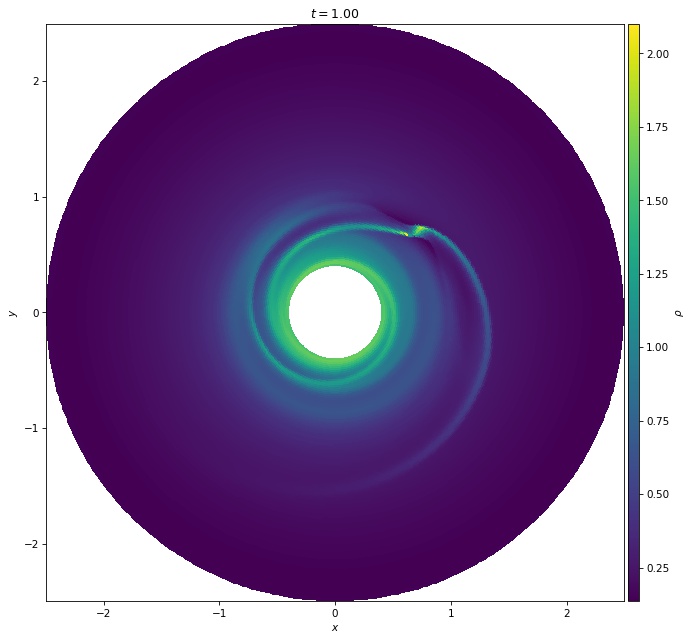
The PlutoData object provides a plot() function, which will automatically project the data onto a cartesian grid, and annotating the axes and colorbar correctly:

sim[-1].plot('rho')

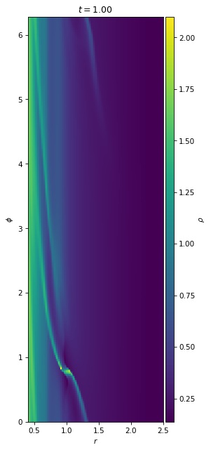
The projection can also be turned off, an arbitrary options which will be passed to matplotlib can be given:

sim[-1].plot('rho', projection=False)

If a plot of a custom quantitity is needed, a array instead of a variable name can be given:

step = sim[-1]
step.plot(step.prs / step.rho, label="T")

In Jupyter Notebooks interactive plotting can be used to step through the simulation steps. Simulation.iplot() has the same interface as PlutoData.plot(), but it will show a slider to step through simulation steps:

sim.iplot("rho")